
When you hear the term ‘ranges of outcomes’ what does it mean to you? I wonder if it has become a term often used and rarely understood.
If I say X has a range of outcomes between zero and 20 what does that mean? Is zero just as likely to hit as 20? Is the most likely outcome in the middle of that range? Thinking in terms of ranges of outcomes is an integral part of fantasy football, but to do so effectively you have to understand the unique components of each player’s range.
In this edition of Thinking About Thinking I continue my series addressing probabilistic fantasy football strategy. Each article I will unpack ways our brains work in irrational ways that create value in your fantasy football leagues. Last week I discussed analytical prospect models, and the importance of humility when evaluating rookies. If you haven’t yet, make sure to check that out to get a feel for this series!
Tua Be or Not Tua Be?
I recently posted a twitter thread about Tua Tagovailoa after Tyreek Hill‘s trade to the Dolphins. In it I discussed the difference between a large scale change to his ranges of outcomes vs. a series of small shifts to each outcome within his range. My belief is that Hill’s addition is more the later than the former.
My next 'Thinking About Thinking' will be about ranges of outcomes & the difference b/w changes to the range vs. changes in probability along the range
▶️ Tua: the determining factor of his dynasty value remains 'is he good?' Tyreek doesn't massively change this..
THREAD:
— Jakob Sanderson (@JakobSanderson) March 23, 2022
What does this mean? We’ll come back to that. First let’s talk about what a range of outcomes is, how it’s created, the types of ranges we often see in fantasy football, and how they are modified. We will discuss this with…
Another Fricking Analogy
I often start theory-heavy articles with an analogy removed from football. I do this for a few reasons. First, the elements of probabilistic thinking which manifest in fantasy football appear often in our every day lives. Second, fantasy gamers carry entrenched priors about given players. It is much easier when trying to build consensus to first agree on a premise, and then extend that premise to your desired position. If you target a position directly, the natural instinct is to find ways to disagree with any premise which leads to this dissonance. After all, I am just one irrational creature of emotion speaking to several others, trying to agree about a fake football game.
The Wheels on the Bus
The Analogy du jour centres on something I know very well; waiting at the bus stop.
Each day you start work at 9:00 AM, and it takes on average 30 minutes for the bus to get to work while making no stops along the way. A new bus leaves your stop every minute. It takes you fifteen minutes on average to walk to the bus. Thus, on average, you will be on time for work if you leave your house at 8:15 AM or earlier. However, we know that is not a certainty.
The ranges of outcomes in this scenario is driven by the speed of your walk, and the speed of the bus on route to work. The ranges of outcomes for how long it takes to get to work probably looks like this.
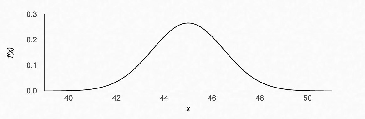
In the above distribution, the total travel time is along the bottom, X-axis, and the probability of each given amount of time is along the side, Y-axis. We see a range between 40 and 50 minutes with a median outcome of 45 minutes. You are no more likely to be early than late.
The Normal Distribution isn’t Always Normal
The above curve is called a ‘normal’ distribution. However, we know this is not an accurate depiction of how your commute actually works. Busses are scheduled at set intervals. If your bus leaves every 10 minutes, the distribution of your ranges of outcomes becomes much less smooth. In the first outcome, no matter when you arrive at the stop, you now have a normally distributed commute at median 30 minutes to work. Any change in arrival time at the stop has the same expected impact on arrival time.
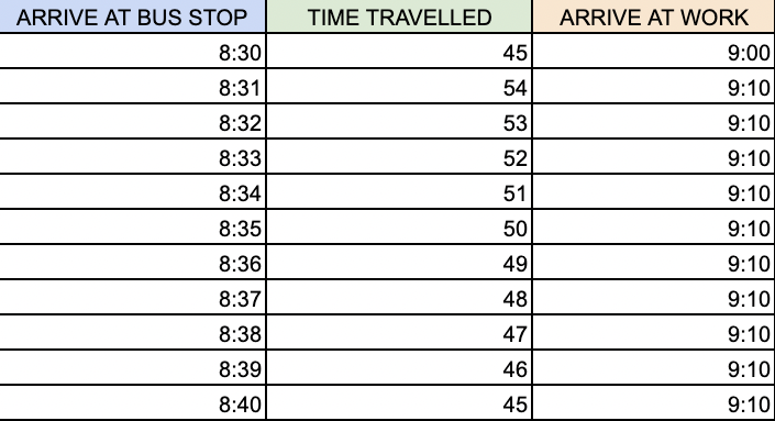
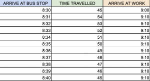
When you account for intervals of bus departure this changes. If the bus leaves at 8:30 and 8:40, there is no change in expected arrival time if you arrive at the stop at 8:31 or 8:39. The inputs in the distribution now look like this:
Stretches, Shifts, Asymmetry and Multi-Modality
Extending this bus example, I want to talk through four ways a distribution can be modified that appear generally in fantasy football.
Stretches
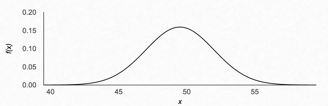
Assuming you are equally likely to show up to the bus stop at any given time, the distribution on time travelled now looks like this. Previously, the only inputs were walking time and bussing time. Now we’ve included wait time, which has the effect of stretching the curve to the right. The minimum time travelled is the same as in the first curve, but the median time and maximum time is higher. The range of outcomes is wider, and the probability of any given time interval is lower.
Shifts
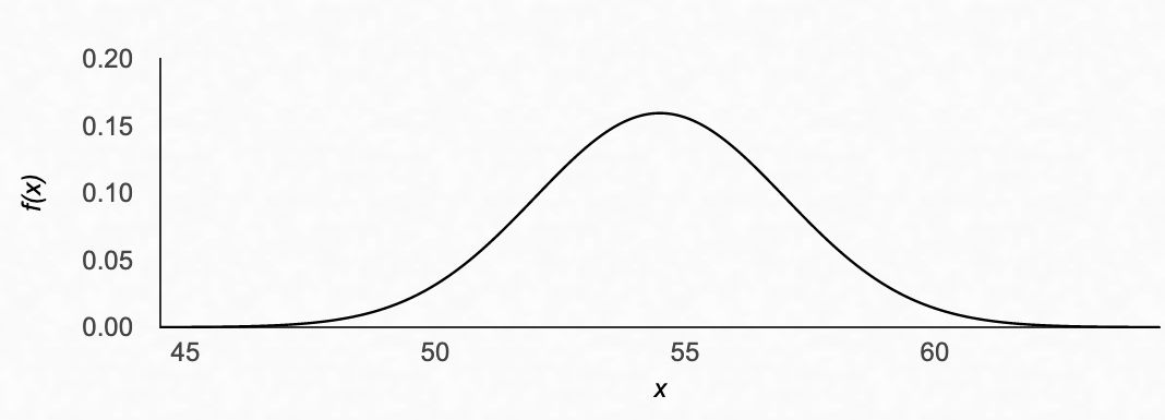
Ok now let’s say there’s construction on your rote, adding on average five minutes to your commute. This change, diagrammed below, shows this effect. The distribution curve is the same as above, but it is shifted to the right.
Asymmetry
Let’s combine these scenarios together.
First, you are aware of the time the bus comes, and thus aim to arrive exactly at 8:30. For that reason, it is most likely you will show up at or near 8:30, not miss your bus, and take closer to 45 minutes to work than the upper ranges.
Second, let’s say the construction does not begin until 9:00AM. Thus, if you are on time for the bus you will likely avoid it. However, if you are on the later bus, your travel time will be lengthened further. We now see a curve that will look roughly like this.

Here is what this shape of curve now reflects:
- The range of outcomes has been expanded due to the possibility of either avoiding or hitting traffic depending on when you catch the bus
- The probability along the distribution is highest around the optimal travel time because you know what time the bus leaves
- The right tail is elongated because the length of travel time increases on the later bus due to construction is combined with the time waiting at the bus stop if you are late
This is the type of curve to envision when you hear “asymmetrical upside” in fantasy football.
Multi-Modality
The final curve type I want to discuss today is the mutli-modal curve. A modal outcome is a most likely outcome: this is different from the median outcome (the outcome in which an equal number of outcomes are better or worse), or the mean outcome; the average.
So what does ‘multi-modal’ mean?
It is a probability distribution that merges two curves with two different outcomes. Let’s look back at this chart.
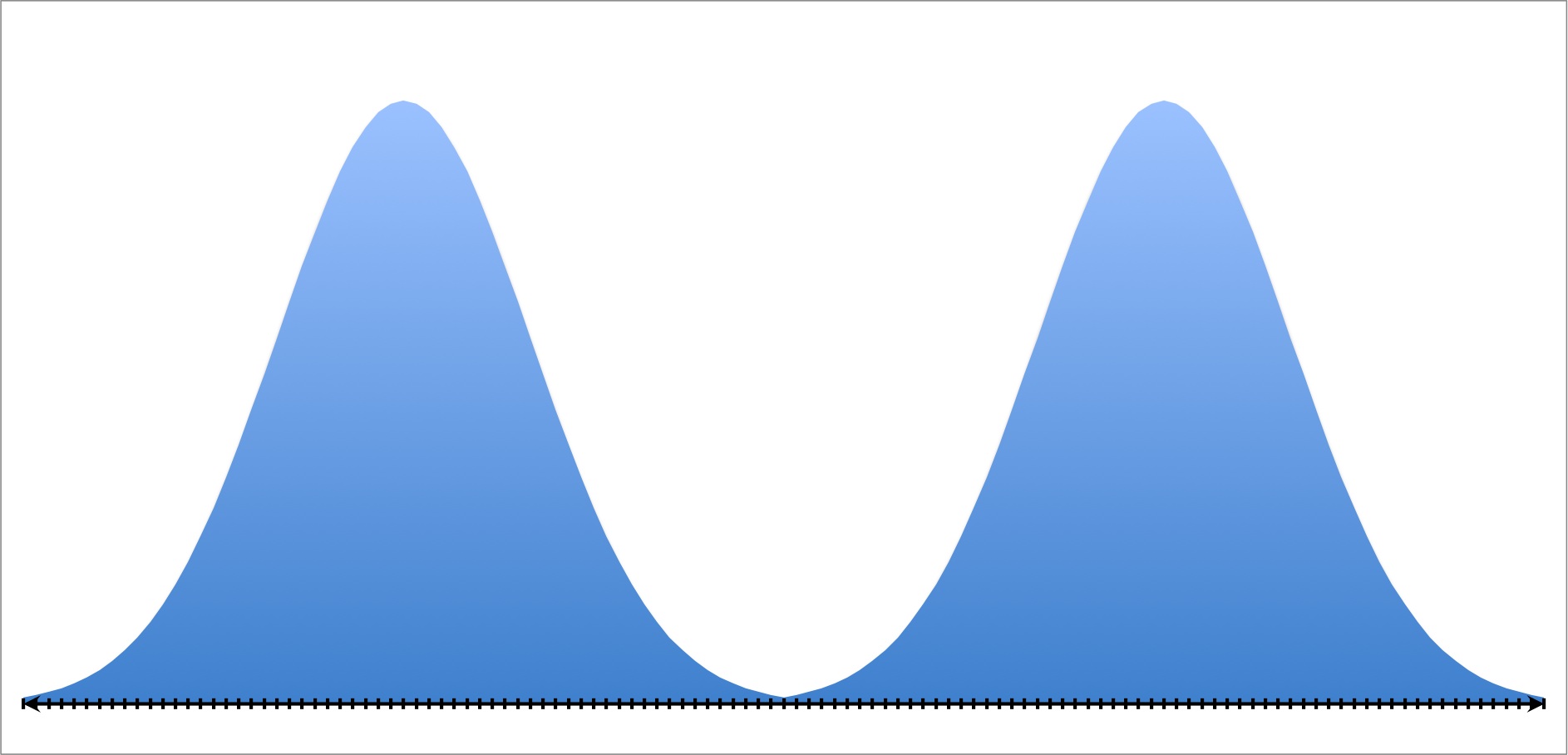
What would it look like if instead of modelling the time travelled we modelled the time of arrival? This would be a multi-modal distribution.
Depending on which bus you catch, each has a normally distributed arrival time in ten minute intervals. The time of arrival curve, if you show up to the bus stop between 8:21 and 8:40 would look roughly like this.
An Actual Football Application
This is a very common distribution idea in fantasy football. Consider Alexander Mattison. In games Dalvin Cook missed, he averaged 22.45 points per game. In all other games he surpassed six fantasy points just once.
Mattison’s distribution is largely bimodal. His ranges of outcomes in a given season are an amalgamation of his range with Cook healthy, his range if Cook is injured, and the likelihood of such an injury.
Mattison last year averaged 8.06 points per game yet rarely scored close to that number. That’s because of his distribution.
Eight fantasy points was an unlikely ceiling for his weeks with Cook, and an unlikely floor in weeks without. His curve would look something like this. As you see below, his distribution is both bi-modal and asymmetrical.

How Do We Use these in Fantasy Football?
Just as there is in our bus example, the distribution of outcomes is rarely simple, and there are numerous inputs at play. But that doesn’t mean understanding these concepts isn’t helpful. Let’s return to the example of Tua Tagovailoa and how to view him in the context of the Tyreek Hill trade.
Before we address the effect of the Hill trade let’s talk about how to view Tagovailoa as an asset, particularly in dynasty.
Young Players are Largely Bi-Modal in Dynasty
Whenever you draft a young player in dynasty you are doing so for two reasons. Firstly, they have the ability to be productive on your team far longer than a veteran. Secondly, they have a higher value ceiling if they hit than a veteran because of their youth.
How does this manifest in terms of their distribution curves? The increased uncertainty as to the player’s ability is a stretch, indicating a wide range of outcomes. The extended value ceiling often creates ranges which are asymmetrically positive; i.e. the ceiling outcome extends disproportionately far beyond the median. The disproportionality between ceiling and median is greatest on lower-drafted options with far lower expectations and median outcomes.
I also want to note that I am NOT talking about asymmetrical upside as it relates to the cost of acquisition. I will explore that in my next article of the series.
Why do I say young players’ distributions are bi-modal?
Because longevity is a function of talent.
If you were to plot the lifetime value of a rookie quarterback entering the league, the ranges of outcomes on that value is an aggregation of all possible outcomes in their career. Most notably: are they good enough at football to have a long career? We could then calculate all varying degrees of ‘good’ or ‘bad,’ how their team responds to negative play, and how productive they are for fantasy in each outcome. But let’s focus first on the blunt, general, question: is the player good enough to have a long NFL career?
Assessing Tua Tagovailoa’s Career
As it pertains to Tua Tagovailoa, the question of his talent remains unknown.
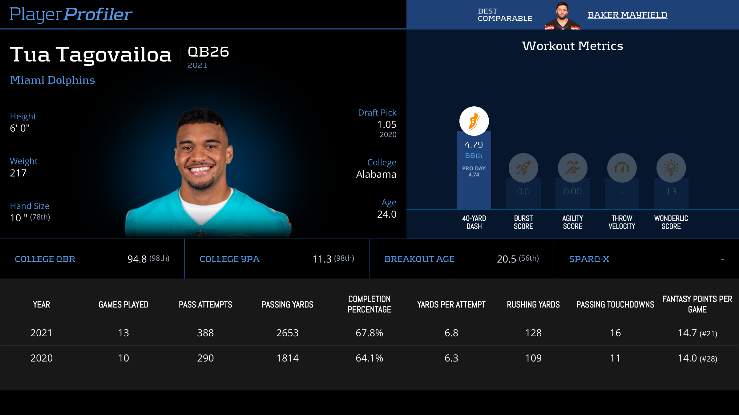
The former Alabama pivot has been a mixed-bag through his first two years in the league. Noted for his ball placement, Tagovailoa ranked third and first in Accuracy Rating. However, he sits 23rd in Yards Per Attempt, and had just 22 Money Throws compared to 31 Danger Plays. While analysts have wide-ranging priors on Tagovailoa, no-one should have certainty regarding the 2017 National Champion’s career trajectory.
Because of the uncertainty in his profile, Tagovailoa’s dynasty value depends heavily upon how he performs as a quarterback this year. Will he prove himself worthy of a second contract as a long-term starter?
Assessing Tua Tagovailoa’s Market Price
Per the dynasty market-evaluation site Keep Trade Cut, Tua Tagovailoa is currently QB18. More importantly, he sits in a tier from QB14-20, negligibly behind tier-mates Aaron Rodgers, Jalen Hurts, and Derek Carr. The gap between the Dolphins quarterback and these three options is much more substantial in seasonal leagues, per Underdog best ball ADP.
Thus, it stands to reason his dynasty price factors in elements of longevity and improvement. In a ceiling scenario, Tagovailoa is a top-12 quarterback this year with his new weapons, entrenching himself as Miami’s franchise quarterback. On the other hand, he could fail to meet expectations and carry precarious job security into 2023.
Schrodinger’s Tua is both alive and dead, but his cost resides in purgatory.
His market value is a compromise position between two plausible outcomes which attempts to balance them appropriately.
How To Evaluate Tyreek Hill’s Impact
There is no question adding Tyreek Hill is a boon to his pivot’s prospects. He is an elite deep threat, separator and yards after catch option who is sure to raise the efficiency of any iteration of Tua Tagovailoa in 2022.
Hill may make good Tua better or bad Tua serviceable, but the primary ballot holder in Tagovailoa’s referendum year is the QB himself. For that reason, any material increase in the quarterback’s dynasty market is likely inefficient. Tagovailoa is already up 6.5-percent on Keep Trade Cut since the trade and may continue rising. Whether his pre-trade price was efficient comes down to your priors. This is a strategy column not a football one, so we will hardly discuss those here. What I will say instead, is the delta between your priors on Tua pre and post trade should probably be lower than the delta in his market cost.
What we should be focusing on are any indica as to which of his curves he’s riding on when the season resumes. Is he a long-term quarterback with new weapons and increasing upside? Or is he a short-term QB2 biding his time until the hatchet drops? Hill can be a driver of this to some extent, but it is highly unlikely he is the determinative factor.
Instead, Hill represents an array of marginal, positive shifts along Tagovailoa’s distribution curve making each outcome a little bit better.
While it is entirely plausible Tagovailoa exceeds his current market cost this year, the portion of that likelihood owed to Hill is unlikely to meet his impact on cost of acquisition. Put another way, if we look back and see Tua as a top-10 dynasty quarterback at this time next year, it probably didn’t happen because the Dolphins traded for Tyreek Hill.
How to Weaponize this Distribution in your Leagues
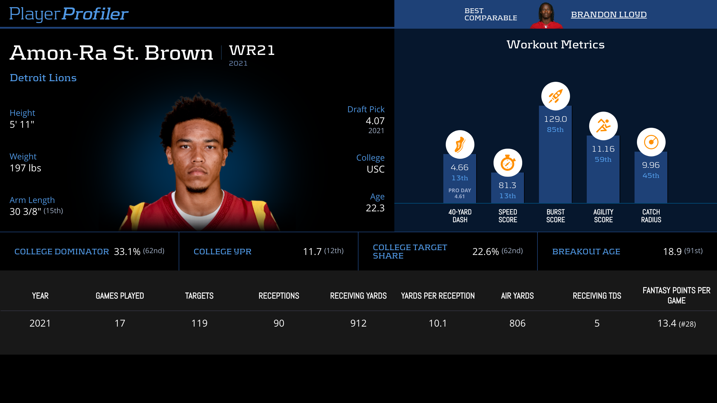
This year we are faced with several young wide receivers coming off promising seasons but likely to be faced with target competition in the draft. The notion of this bi-modality is most relevant with players such as Amon-Ra St. Brown or Darnell Mooney. Because the market is unsure as to their talent level despite strong peripheral usage, large shifts may occur if early draft capital is spent at receiver. Instead of thinking in terms of near-term projection, think in reverse.
Assume the best and worst case scenarios for these players. If we look back two years from now and St. Brown is a top 12 receiver, how many rookies in this class could have prevented that breakout from happening? If in two years Mooney is an afterthought, what are the odds a round two rookie is the reason why?
Could target competition matter at the margins for these players? Absolutely. However, it is unlikely that at the most impactful ends of their range – positive and negative – the added target competition is determinative of their career trajectory. For this reason, if either faces a price decrease due to further off-season additions, you should probably be buying if all else is equal.
The Final Word
If you just read through 2,200 words about distribution curves and are relieved it’s over, first of all congrats! Second of all, this is certainly not the last you’ll hear of it in this column. Understanding how players’ value is stored and what inputs change their ranges make us more critical fantasy players. It allows us to gain edges on the margins regardless of our priors. Next time, I will return to the idea of asymmetrical distributions to examine how they presents in fantasy football, when it is factored in by cost, and when we can exploit them.